Summary:
Modify WBTC-long and wstETH-long LlamaLend market min/max rates in the Monetary Policy over multiple steps. The final rates are given below:
| Market | Optimal Utilization (u_opt) |
Recommended rate_min |
Recommended rate_max |
|---|---|---|---|
| wBTC-long | 0.83 | 1.12406e-07 |
0.734 |
| wstETH-long | 0.85 | 3.08e-07 |
0.792 |
Abstract:
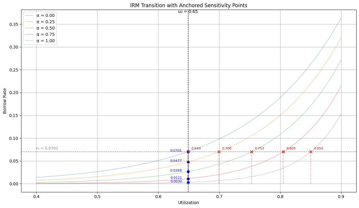
Rate modification is done in steps to minimize impact to the markets over the transition period. Rate modification at each step is given below:
WBTC
| Step | α | PredRate@u₀ | PredUtil@r₀ | rate_min | rate_max |
|---|---|---|---|---|---|
| 0 | 0.00 | 0.07014 | 0.65 | 0.0010000841581024266 | 0.6999883263876364 |
| 1 | 0.25 | 0.04768 | 0.70 | 0.00034804412367539224 | 0.683586885074309 |
| 2 | 0.50 | 0.02678 | 0.75 | 0.00006759457428125955 | 0.6819674901911611 |
| 3 | 0.75 | 0.01105 | 0.81 | 0.00000520029461078648 | 0.6988885299433425 |
| 4 | 1.00 | 0.00297 | 0.85 | 0.00000011240581253764277 | 0.733678930058516 |
wstETH
| Step | α | PredRate@u₀ | PredUtil@r₀ | rate_min | rate_max |
|---|---|---|---|---|---|
| 0 | 0.00 | 0.04115 | 0.52 | 0.002000141964376983 | 0.699989161244529 |
| 1 | 0.20 | 0.02811 | 0.57 | 0.0009187163953148215 | 0.6933587924725291 |
| 2 | 0.40 | 0.01648 | 0.63 | 0.0003025976088515107 | 0.6975366924396146 |
| 3 | 0.60 | 0.00768 | 0.70 | 0.00006079056373688122 | 0.7153441443752199 |
| 4 | 0.80 | 0.00266 | 0.75 | 0.000006481614380540609 | 0.746925353699179 |
| 5 | 1.00 | 0.00063 | 0.80 | 0.0000003082574640293203 | 0.7919310470189376 |
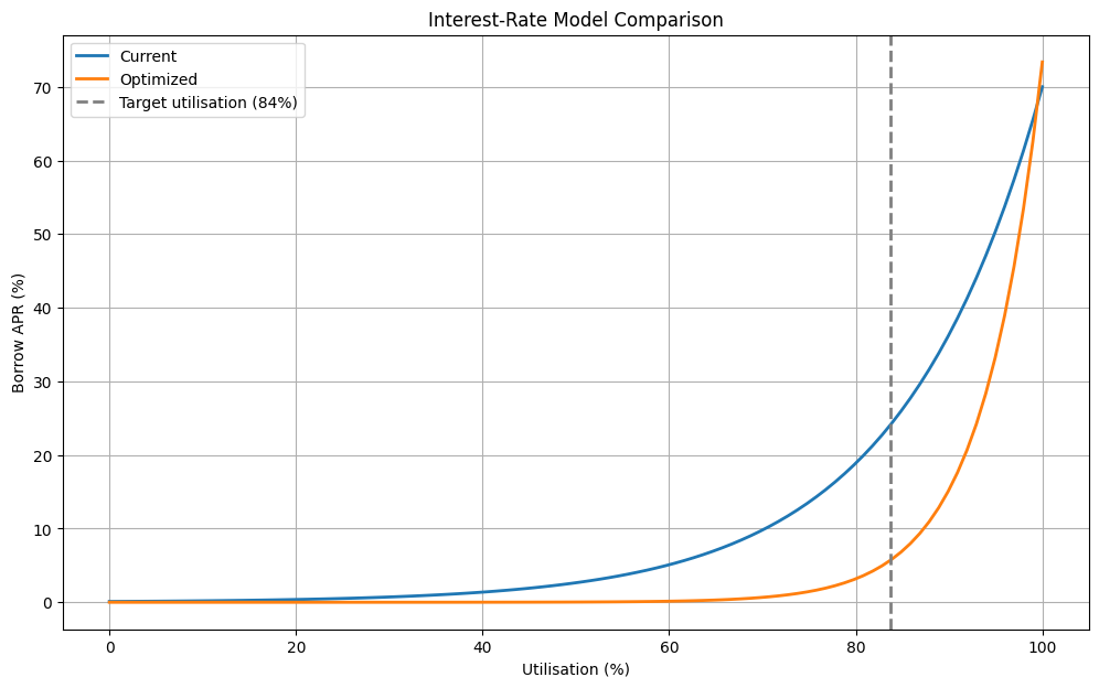
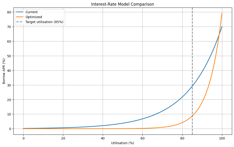
Motivation:
This vote will modify the interest rate curve for the target markets. The goal is to improve market performance by improving the equilibrium utilization while protecting both lenders and borrowers with reasonable liquidity assurances and rate volatility. Our analysis below supports the transition plan given above.
Analysis:
Market: wBTC-long
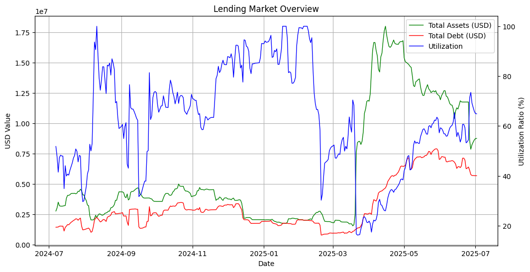
Optimal Utilization
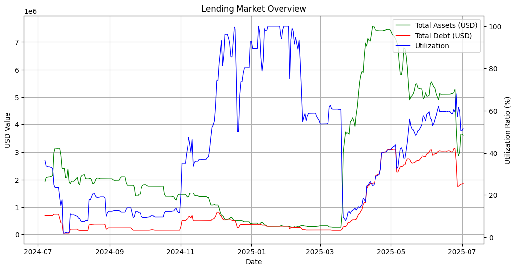
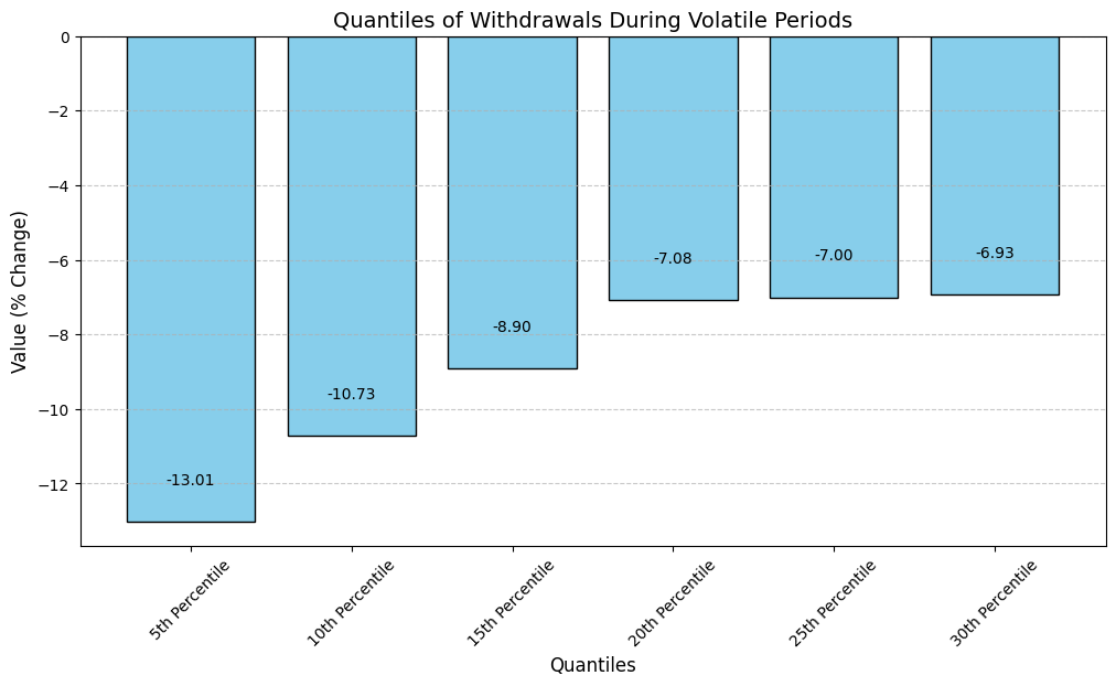
We estimate the optimal utilization threshold for the WBTC market by analyzing historical withdrawal behavior during volatile price periods.
Methodology
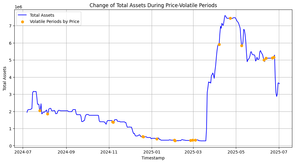
- Volatile periods are defined as days when the oracle price changes exceed 2× the standard deviation.
- During these periods, we focus on negative changes in total assets to capture actual withdrawals.
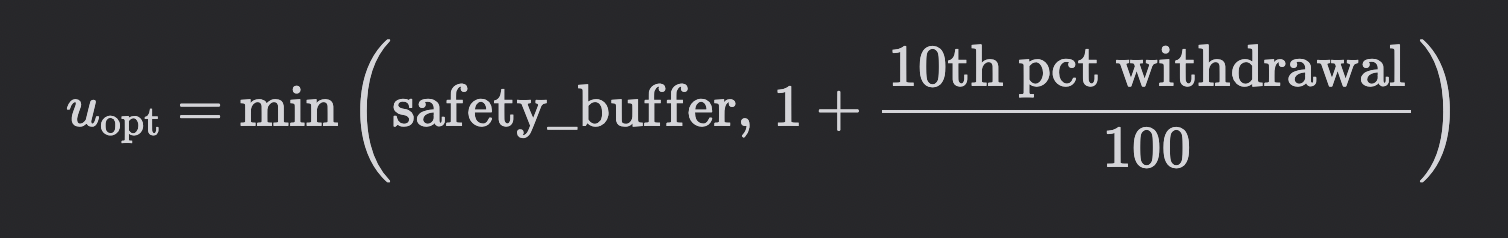
- The 10th percentile of these withdrawals is used to define a safety buffer for utilization.
- A conservative safety buffer cap of 85% ensures that utilization does not exceed a level that might trigger liquidity stress during adverse events.
Results
| Yellow dots mark volatile price days where withdrawal behavior is evaluated. | Distribution of asset drawdowns in volatile windows. The 10th percentile determines u_opt. |

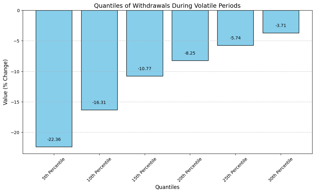
The Findings suggest an optimal utilization of 0.83 for the WBTC market.
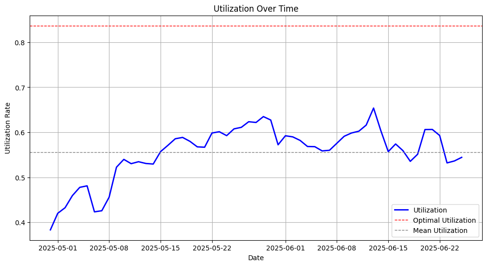
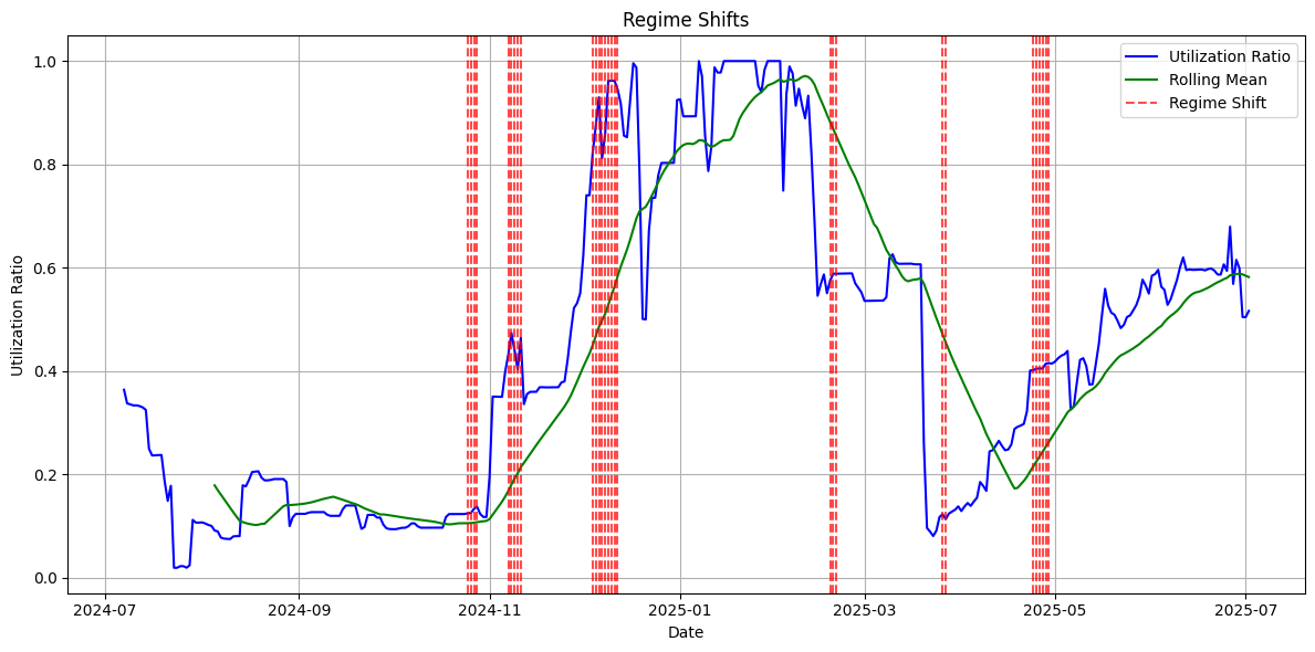
Regime
We apply a rolling Z-score-based method to identify stable utilization behavior in the WBTC market. A regime is confirmed when utilization deviates beyond 1.5 standard deviations for 7 consecutive days.
Detected Regime
- Start: 2025-04-29
- End: 2025-06-26
- Classification: Transition from fluctuating to stable utilization behavior, approaching target levels
| Z-score deviations indicate entry into a stable regime. | Within this window, utilization stabilizes closer to the optimal target (u_opt = 0.83). |
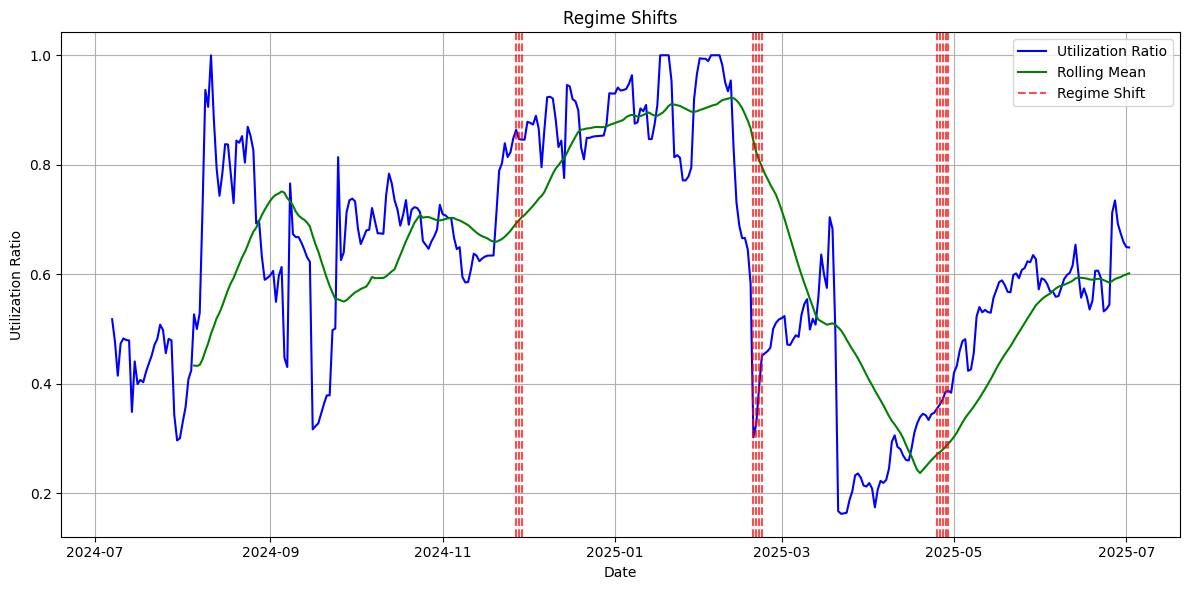
Note on data argumentation: The WBTC market experienced a recent supply shock likely due to the recent Resupply hack. As the WBTC market, relative to the wstETH and wETH market, was more meaningfully affected in the utilization, we restrict the regime to the 25.06.2025 for this market.
Experiment
Experimental Context
Empirical Estimation of Utilization Sensitivity
To estimate the responsiveness of utilization to changes in the borrow rate, we employed a 2-stage Ordinary Least Squares (OLS) regression. The dependent variable is the first-difference of utilization (delta_utilization), and the primary independent variable is the lagged borrow APR (borrow_apr_lag).
OLS Regression Results
==============================================================================
Dep. Variable:      delta_utilization   R-squared:                       0.138
Model:                            OLS   Adj. R-squared:                  0.124
Method:                 Least Squares   F-statistic:                     9.465
Date:                Wed, 02 Jul 2025   Prob (F-statistic):            0.00317
Time:                        21:37:49   Log-Likelihood:                 145.39
No. Observations:                  61   AIC:                            -286.8
Df Residuals:                      59   BIC:                            -282.5
Df Model:                           1
Covariance Type:            nonrobust
==================================================================================
                     coef    std err          t      P>|t|      [0.025      0.975]
----------------------------------------------------------------------------------
const              0.0219      0.007      2.964      0.004       0.007       0.037
borrow_apr_lag    -0.4443      0.144     -3.077      0.003      -0.733      -0.155
==============================================================================
Omnibus:                        9.037   Durbin-Watson:                   1.741
Prob(Omnibus):                  0.011   Jarque-Bera (JB):               10.783
Skew:                          -0.588   Prob(JB):                      0.00455
Kurtosis:                       4.691   Cond. No.                         49.8
==============================================================================

Notes:
[1] Standard Errors assume that the covariance matrix of the errors is correctly specified.
Moment Matching Validation
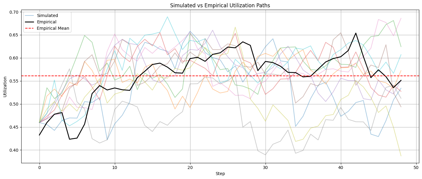
We validate the simulation’s realism by comparing empirical and simulated utilization moments:
| Moment | Empirical | Simulated | Δ (Sim – Emp) |
|---|---|---|---|
| Mean | 0.561 | 0.563 | +0.002 |
| Std. Dev. | 0.054 | 0.055 | +0.001 |
| Skewness | -0.523 | -0.431 | +0.092 |
| Kurtosis | 1.575 | 1.559 | -0.016 |
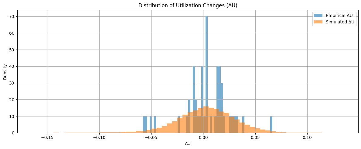
| Simulated utilization paths exhibit behavior consistent with the observed regime. | Simulated distribution closely matches empirical shape. |
Experiment
We optimize the IRM within the detected stable regime to improve alignment with target utilization.
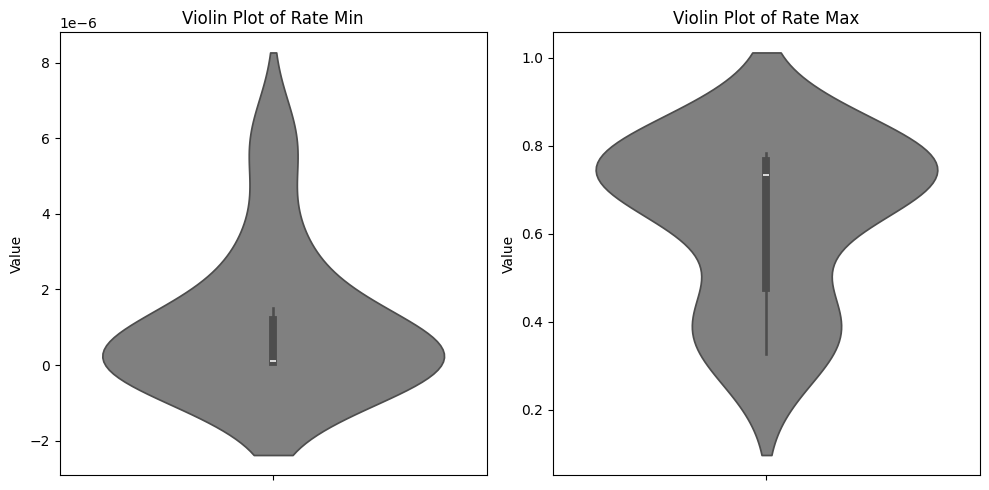
Optimizer Stability
We conduct multiple optimization runs are conducted with varying seeds to ensure robustness.
The median parameter set is selected for final recommendation:
![]()
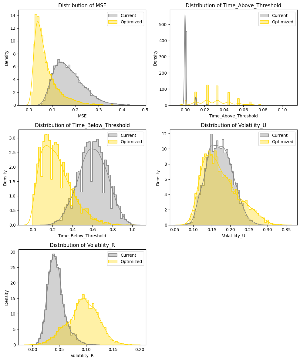
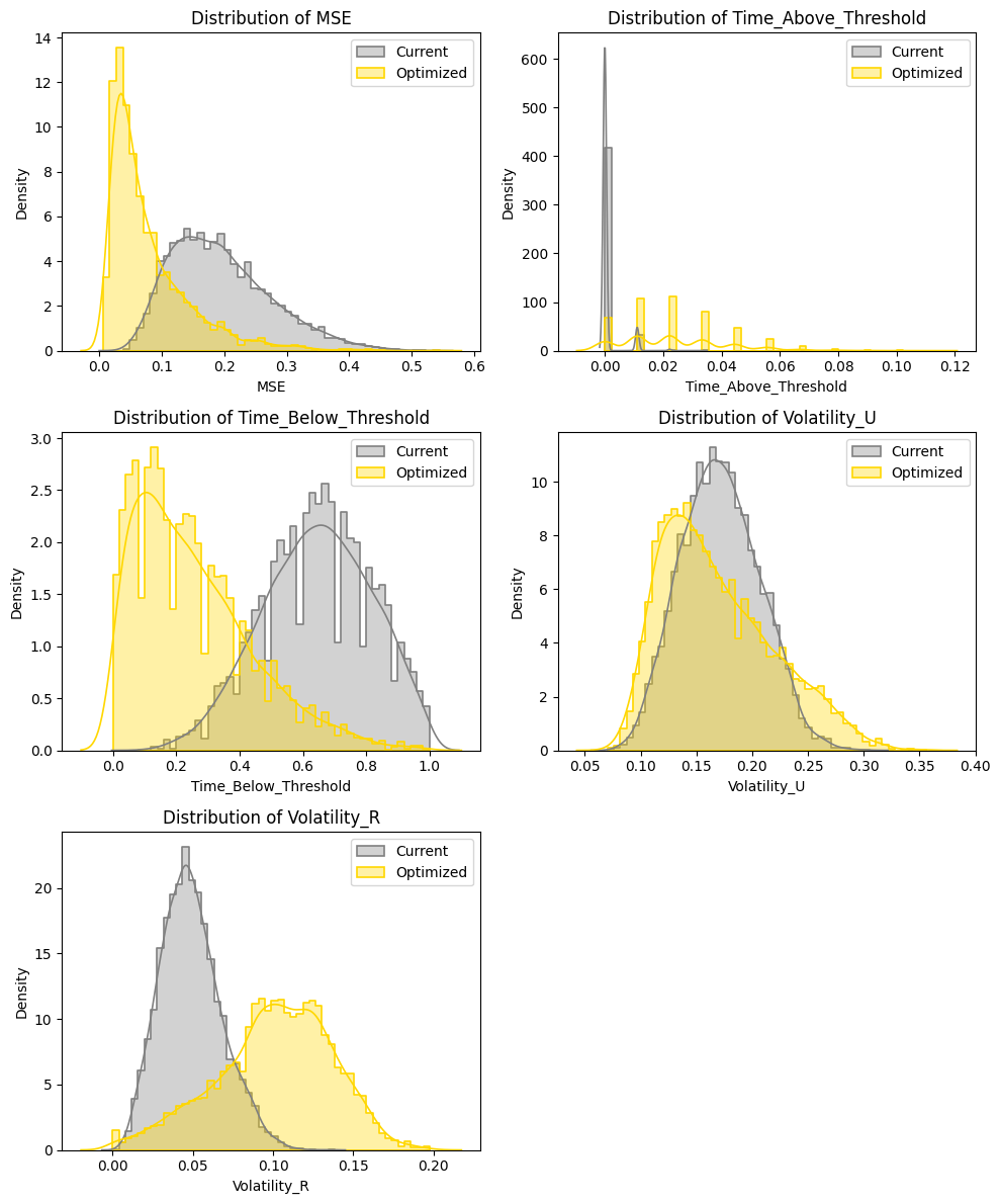
Performance Evaluation
Performance is evaluated relative to the existing policy across simulated paths under the current regime.
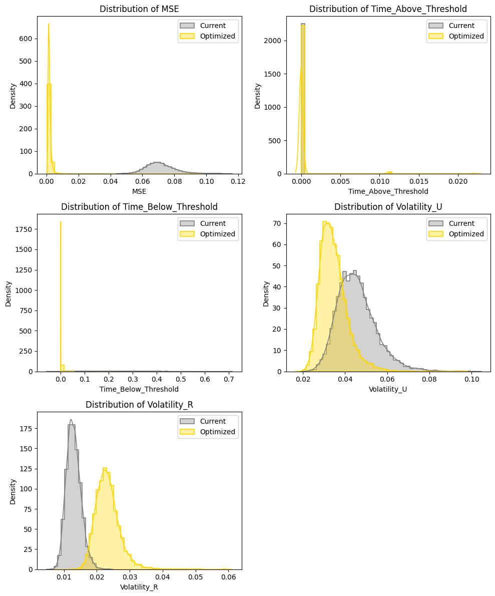
Key Observations:
- MSE: Meaningfully lower compared to the current production implementation.
- Time Above Threshold: Similar performance with a few days of simulated paths spending in utilization above 93%.
- Time Below Threshold: Concentrate at the lower end with barely any paths spending time below 53% utilization.
- Utilization Volatility: Stablises indicating lower volatility.
- Rate Volatility: Increases compared to production implementation.
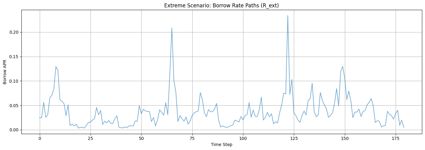
Stress Test: Extreme Events
To evaluate the IRM under tail-risk conditions, we simulate extreme market scenarios using scaled historical volatility and jump behavior.
Methodology
- Volatility scaled by 1.5×
- Jump size increased by 2.0×
- Jump frequency increased by 1.5×
- Tail exponent (ν) reduced to simulate fatter tails
A total of 500 stress paths were generated using the optimized IRM under these scaled conditions.
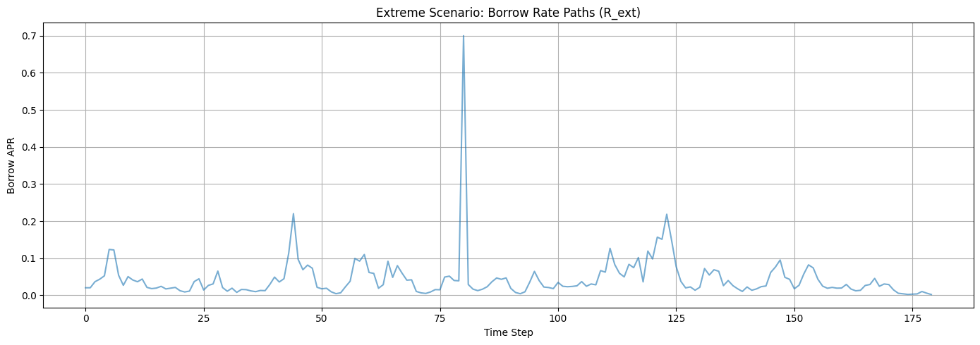
Illustrative Scenario Example under current IRM parameters
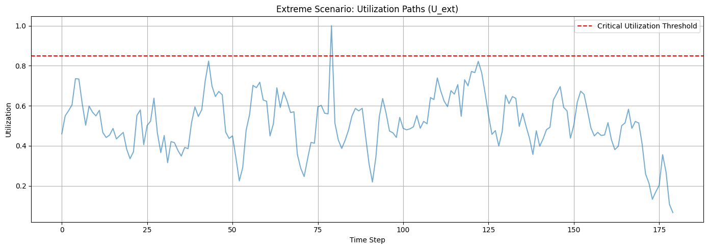
Performance Evaluation
| The IRM maintains acceptable performance under stress, with moderate volatility and bounded risk exposure. |
Key Observations
- Lower MSE: The optimized IRM continues to track target utilization more closely, even under extreme conditions.
- Higher Peak Utilization: Up to 10% of the simulated horizon exceeds the 95% threshold — a trade-off for responsiveness.
- Reduced Underutilization: Time spent below critical levels remains meaningfully lower than baseline.
- Utilization Stability: Lower mean volatility, though with a wider distribution, however equally wide distribution.
- Borrow Rate Behavior: Rates exhibit a wider distribution and higher volatility, reflecting the IRM’s adaptive response to extreme shifts.
Recommendation
We recommend following parameter for a Semilog implementation:
- rate_min = 1.12406e-07
- rate_max = 0.73368
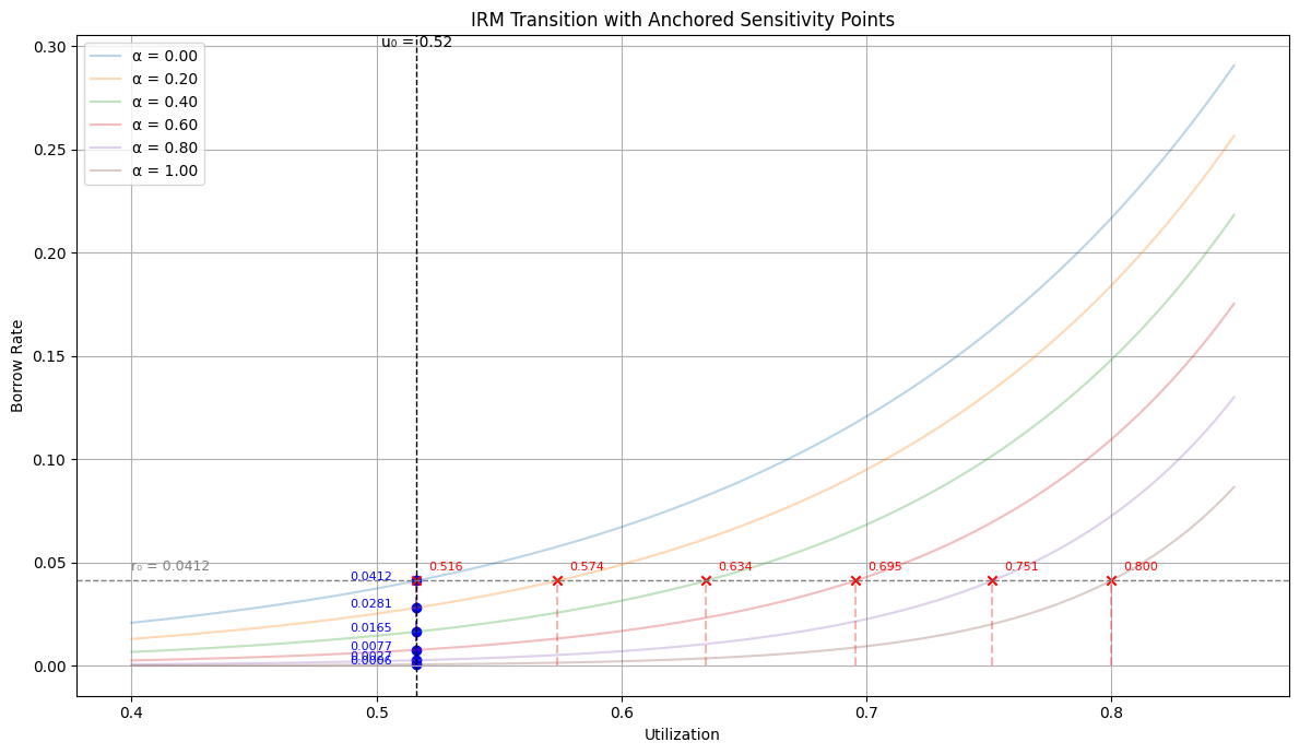
Transition Management
Stepwise Transition Summary
| Step | α | PredRate@u₀ | PredUtil@r₀ | rate_min | rate_max |
|---|---|---|---|---|---|
| 0 | 0.00 | 0.07014 | 0.65 | 0.0010000841581024266 | 0.6999883263876364 |
| 1 | 0.25 | 0.04768 | 0.70 | 0.00034804412367539224 | 0.683586885074309 |
| 2 | 0.50 | 0.02678 | 0.75 | 0.00006759457428125955 | 0.6819674901911611 |
| 3 | 0.75 | 0.01105 | 0.81 | 0.00000520029461078648 | 0.6988885299433425 |
| 4 | 1.00 | 0.00297 | 0.85 | 0.00000011240581253764277 | 0.733678930058516 |
Market: wstETH-long
Optimal Utilization
To ensure sufficient capital during stress events, we estimate the optimal utilization (u_opt) using observed withdrawal behavior in volatile periods.
Methodology Re-cap
-
Volatility Detection: Price changes exceeding 2× the standard deviation are flagged as volatile.
-
Withdrawal Quantile: During these periods, we analyze asset drawdowns and extract the 10th percentile of negative withdrawals.
-
Calculation:
With
safety_buffer = 0.85, this ensures a conservative ceiling.
Results
| Volatile periods identified based on price oracle feed. | Distribution of asset withdrawals; 10th percentile marked. |
- Volatility threshold captured meaningful stress periods.
- Estimated
u_opt= 0.85, capped by the safety buffer.
Regime Detection
We identify a stable utilization regime using a rolling z-score detector with a 30-day window and a 1.5 standard deviation threshold. A regime shift is confirmed if utilization deviates beyond this threshold for 7 consecutive days.
| Z-score based detection of abnormal utilization behavior. | Classification of utilization levels during the stable regime relative to u_opt. |
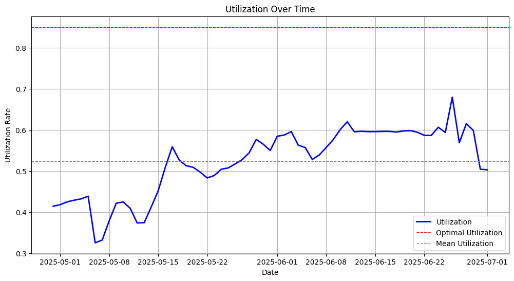
The latest identified regime reaches from the 2025-04-29 to 2025-07-02. It can be classifed as underutilized relative to u_opt.
Experiment
Experimental Context
Empirical Estimation of Utilization Sensitivity
To estimate the responsiveness of utilization to changes in the borrow rate, we employed a 2-stage Ordinary Least Squares (OLS) regression. The dependent variable is the first-difference of utilization (delta_utilization), and the primary independent variable is the lagged borrow APR (borrow_apr_lag).
OLS Regression Results
==============================================================================
Dep. Variable:      delta_utilization   R-squared:                       0.059
Model:                            OLS   Adj. R-squared:                  0.043
Method:                 Least Squares   F-statistic:                     3.731
Date:                Wed, 02 Jul 2025   Prob (F-statistic):             0.0581
Time:                        12:36:59   Log-Likelihood:                 125.02
No. Observations:                  62   AIC:                            -246.0
Df Residuals:                      60   BIC:                            -241.8
Df Model:                           1
Covariance Type:            nonrobust
==================================================================================
                     coef    std err          t      P>|t|      [0.025      0.975]
----------------------------------------------------------------------------------
const              0.0217      0.011      1.935      0.058      -0.001       0.044
borrow_apr_lag    -0.4175      0.216     -1.932      0.058      -0.850       0.015
==============================================================================
Omnibus:                       24.897   Durbin-Watson:                   2.118
Prob(Omnibus):                  0.000   Jarque-Bera (JB):               60.735
Skew:                          -1.170   Prob(JB):                     6.48e-14
Kurtosis:                       7.247   Cond. No.                         52.1
==============================================================================

Notes:
[1] Standard Errors assume that the covariance matrix of the errors is correctly specified.
The negative and borderline-significant coefficient on borrow_apr_lag suggests an inverse relationship between interest rates and utilization changes, consistent with rational borrower behavior. However, explanatory power remains limited (R² ≈ 6%), highlighting the importance of incorporating simulation-based methods for model tuning.
Moment Matching Validation
To calibrate the IRM and ensure it reproduces realistic utilization dynamics, we validated the simulated utilization paths against empirical moment targets.
Empirical vs. Simulated Moments:
| Moment | Empirical | Simulated | Δ (Sim – Emp) |
|---|---|---|---|
| Mean | 0.5264 | 0.5229 | -0.0035 |
| Std. Dev. | 0.0790 | 0.1031 | +0.0241 |
| Skewness | -1.173 | -1.217 | -0.0445 |
| Kurtosis | 3.647 | 3.780 | +0.1331 |
The simulation accurately reproduces the empirical mean and skew, with slight overestimation in volatility and tail thickness (kurtosis). The match is visually confirmed in the figures below:
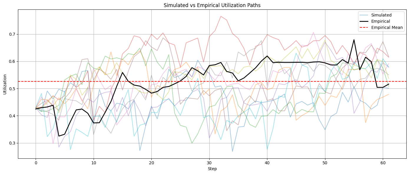
Simulated utilization paths with empirical mean overlay.
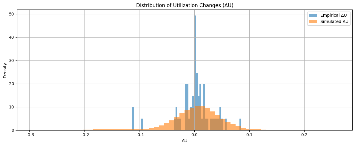
Distributional comparison between simulated and empirical utilization.
IRM Optimization
We optimize the Interest Rate Model (IRM) within the detected regime, comparing performance against the existing policy. To ensure robustness, we:
- Re-run the optimizer 10 times with different random seeds.
- Select the median parameter set across runs as the final recommendation.
- Conduct a stress test using scaled parameters based on historical volatility to validate performance under adverse conditions.
Optimizer Stability:
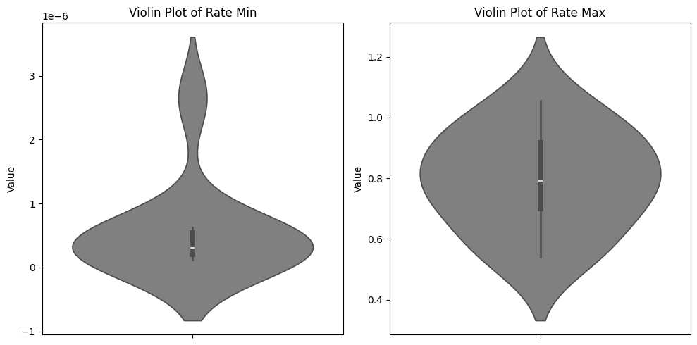
Recommended Parameters (Median):
(rate_min = 3.08e-07, rate_max = 0.792)
Regime Performance Comparison ti Current IRM Configurations:
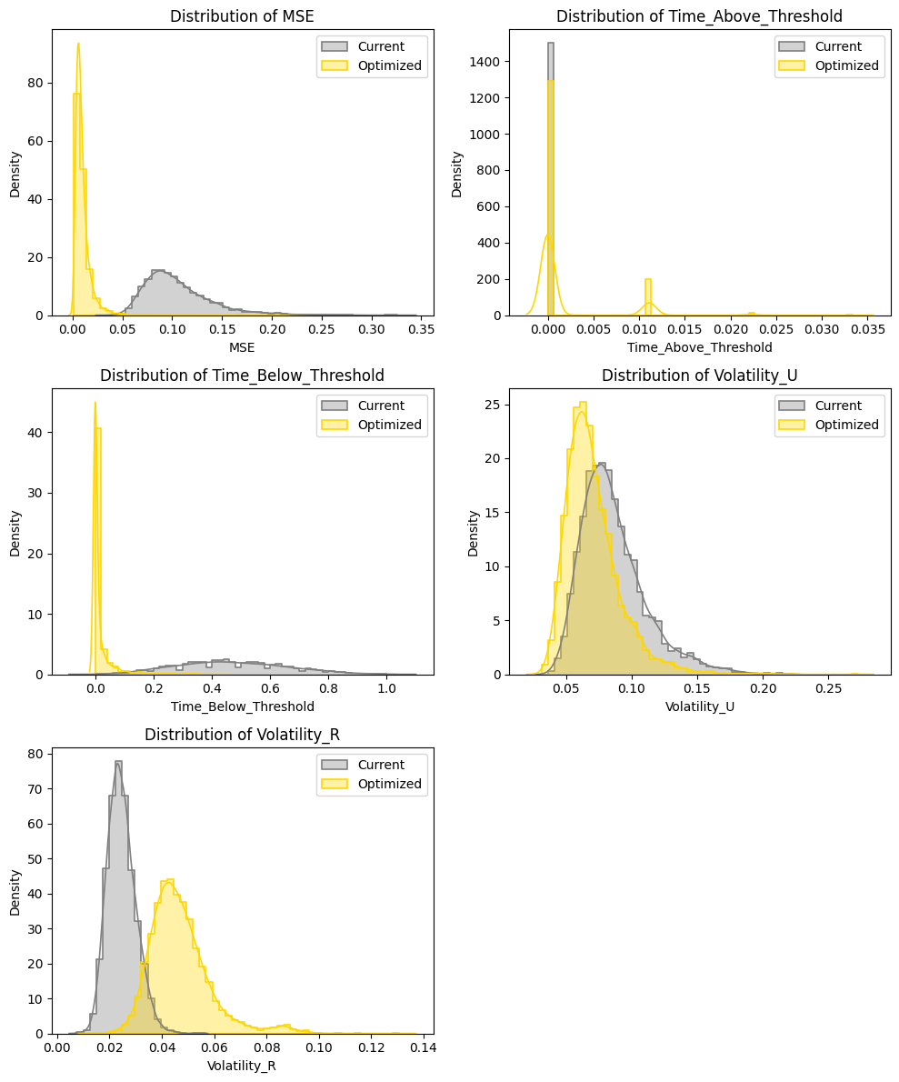
Key Observations
- Lower MSE: The optimized IRM tracks the target utilization more closely than the baseline.
- Improved Capital Efficiency: Only ~3.5% of the simulated period exceeds 95% utilization, indicating minimal overuse risk.
- Reduced Underutilization: Time spent below 55% utilization is meaningfully lower under the optimized IRM.
- Smoother Utilization Path: Slight reduction in utilization volatility, contributing to more stable market conditions.
- Trade-off: The optimized IRM exhibits higher rate volatility, reflecting its increased responsiveness to utilization changes.
Stress Test: Extreme Events
To evaluate the IRM under tail-risk conditions, we simulate extreme market scenarios using scaled historical volatility and jump behavior.
Methodology
- Historical Tail Estimation
We estimate the volatility (σ), jump frequency (p_jump), and jump size (μ_jump) from historical utilization data, identifying deviations beyond 2.5 standard deviations. - Sampler Scaling for Extremes
We modify the base IRM parameters by:- Increasing volatility (1.5×)
- Amplifying jump size (2.0×) and frequency (1.5×)
- Reducing tail exponent
νto simulate fatter tails
- Stress Simulation
500 utilization and rate paths are generated under the modified parameters using the same IRM logic.
Illustrative Scenario Example under current IRM parameters
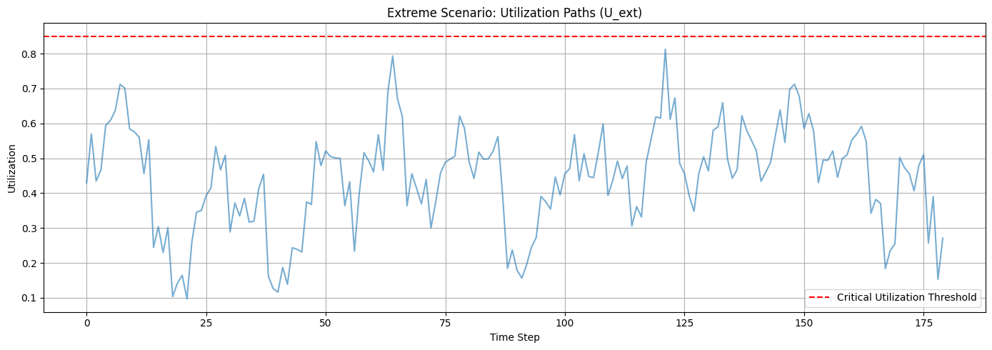
Performance Evaluation
Key Observations
- Lower MSE: The optimized IRM continues to track target utilization more closely, even under extreme conditions.
- Higher Peak Utilization: Up to 12% of the simulated horizon exceeds the 95% threshold — a trade-off for responsiveness.
- Reduced Underutilization: Time spent below critical levels remains meaningfully lower than baseline.
- Utilization Stability: Lower mean volatility, though with a wider distribution, however equally wide distribution.
- Borrow Rate Behavior: Rates exhibit a wider distribution and higher volatility, reflecting the IRM’s adaptive response to extreme shifts.
Recommendation
We recommend following parameter for a Semilog implementation:
- rate_min = 3.08e-07
- rate_max = 0.792
Transition Management
Stepwise Transition Summary
| Step | α | PredRate@u₀ | PredUtil@r₀ | rate_min | rate_max |
|---|---|---|---|---|---|
| 0 | 0.00 | 0.04115 | 0.52 | 0.002000141964376983 | 0.699989161244529 |
| 1 | 0.20 | 0.02811 | 0.57 | 0.0009187163953148215 | 0.6933587924725291 |
| 2 | 0.40 | 0.01648 | 0.63 | 0.0003025976088515107 | 0.6975366924396146 |
| 3 | 0.60 | 0.00768 | 0.70 | 0.00006079056373688122 | 0.7153441443752199 |
| 4 | 0.80 | 0.00266 | 0.75 | 0.000006481614380540609 | 0.746925353699179 |
| 5 | 1.00 | 0.00063 | 0.80 | 0.0000003082574640293203 | 0.7919310470189376 |
Specification
Both markets will require a redeploy of the monetary policy contract with increased bounds (the current contract limits MIN_RATE to 0.1%). A followup post will share the contract address once that has been deployed.