Summary:
Adjust CRV-long LlamaLend market min/max rates from 0.03/466.56% to 0.01817/435.03%.
Abstract:
This vote is intended as a multi-part adjustment to the CRV-long market rates, with minor adjustments toward the target configuration:
| Current | Target | |
|---|---|---|
| Optimal Utilization | 0.65 | 0.82 |
| Rate Min | 0.0003 | 3e-7 |
| Rate Max | 4.66 | 2.93 |
We identify the transition steps by indicating the acceptable level of instantaneous adjustment in rate that we are willing to tolerate and the steps for the adjustment. Below we target an instantaneous adjustment of around ~ 3%.
| Step | α | PredRate@u₀ | PredUtil@r₀ | rate_min | rate_max |
|---|---|---|---|---|---|
| 0 | 0.00 | 0.15914 | 0.65 | 3.000e-04 | 4.6656 |
| 1 | 0.17 | 0.12759 | 0.67 | 1.817e-04 | 4.3503 |
| 2 | 0.33 | 0.09747 | 0.70 | 9.652e-05 | 4.0416 |
| 3 | 0.50 | 0.06948 | 0.72 | 4.234e-05 | 3.7421 |
| 4 | 0.67 | 0.04469 | 0.75 | 1.391e-05 | 3.4550 |
| 5 | 0.83 | 0.02452 | 0.78 | 2.915e-06 | 3.1842 |
| 6 | 1.00 | 0.01049 | 0.82 | 3.000e-07 | 2.9330 |
A visual represention for each policy is show by its α value.
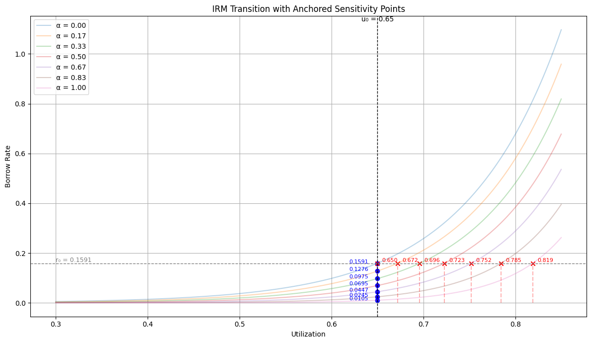
Note: This is a cropped version of the utilization chart to show the most relevant area.
Motivation:
The Monetary Policy parameters are currently set quite conservatively due to historical instability in this particular market. We believe the market to show a healthy demand trajectory and can reduce restrictions on the market’s growth potential by moving the market’s target utilization up from 65% to 82% over an extended observation period.
To ensure a smooth and economically consistent transition between interest rate models (IRMs), we implement a stepwise adjustment mechanism guided by local sensitivity. Rather than interpolating IRM parameters over time, we define each intermediate step by its implied equilibrium utilization at the current borrow rate.
For each IRM step (i), we compute the utilization (u(i)r₀ ) such that the new IRM yields the current borrow rate r₀ :
𝐼𝑅𝑀⁽ⁱ⁾(𝑢⁽ⁱ⁾𝑟₀) = 𝑟₀
This value serves as a transition trigger . The protocol:
- Proceeds to the next step only when observed utilization exceeds (𝑢⁽ⁱ⁺¹⁾𝑟₀), ensuring that the new policy’s rate aligns with market conditions.
- Pauses adjustment if utilization remains below (𝑢⁽ⁱ⁺¹⁾𝑟₀), avoiding premature rate changes.
- Optionally reverts to a previous step if utilization falls below (𝑢⁽ⁱ⁾𝑟₀), maintaining economic consistency in both directions.
The core idea behind this approach is to align policy changes with actual market behavior. By anchoring each step to the utilization level that justifies the current borrow rate under the next policy, we ensure that interest rate adjustments are not imposed arbitrarily but are triggered only when the market conditions naturally support them.
Note: This assumes there is no fundamental shift in the utilization dynamics of the market.
This approach ensures that rate changes are gradual, market-driven, and never come as a surprise to borrowers.
CRV-long Market Analysis
See in the drop down an analysis we have conducted to justify the target parameter configuration for the CRV-long market.
CRV-long Market Analysis
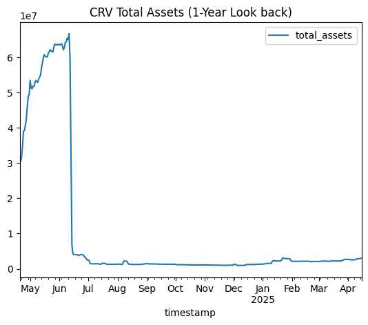
While we recently conducted the CRV-long market, we exclude in this analysis the CRV liquidation event of 140 Million and by starting the analysis after the event.
To contextualize this - we adjust the time series starting from 01-07-2024 instead of an annual lookback window.
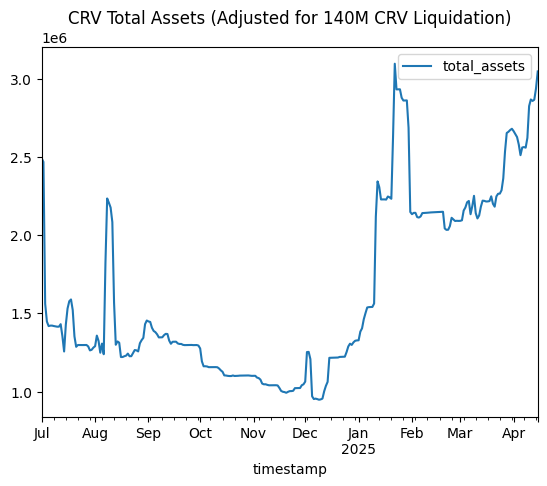
The CRV-long market is deployed with the controller address:0xEdA215b7666936DEd834f76f3fBC6F323295110A.
The current Interest Rate Model (IRM) is SemiLogIRM, with the following parameters following past parameter adjustment:
rate_min=0.0003rate_max=4.66
Optimal Utilization Analysis
We identify volatile periods based on the price oracle feed and then analyze the withdrawal quantile of total assets during these periods.
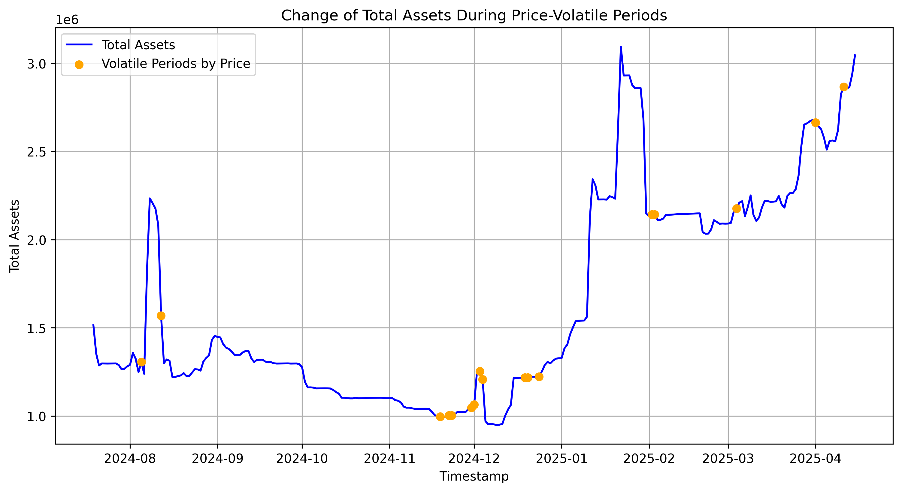
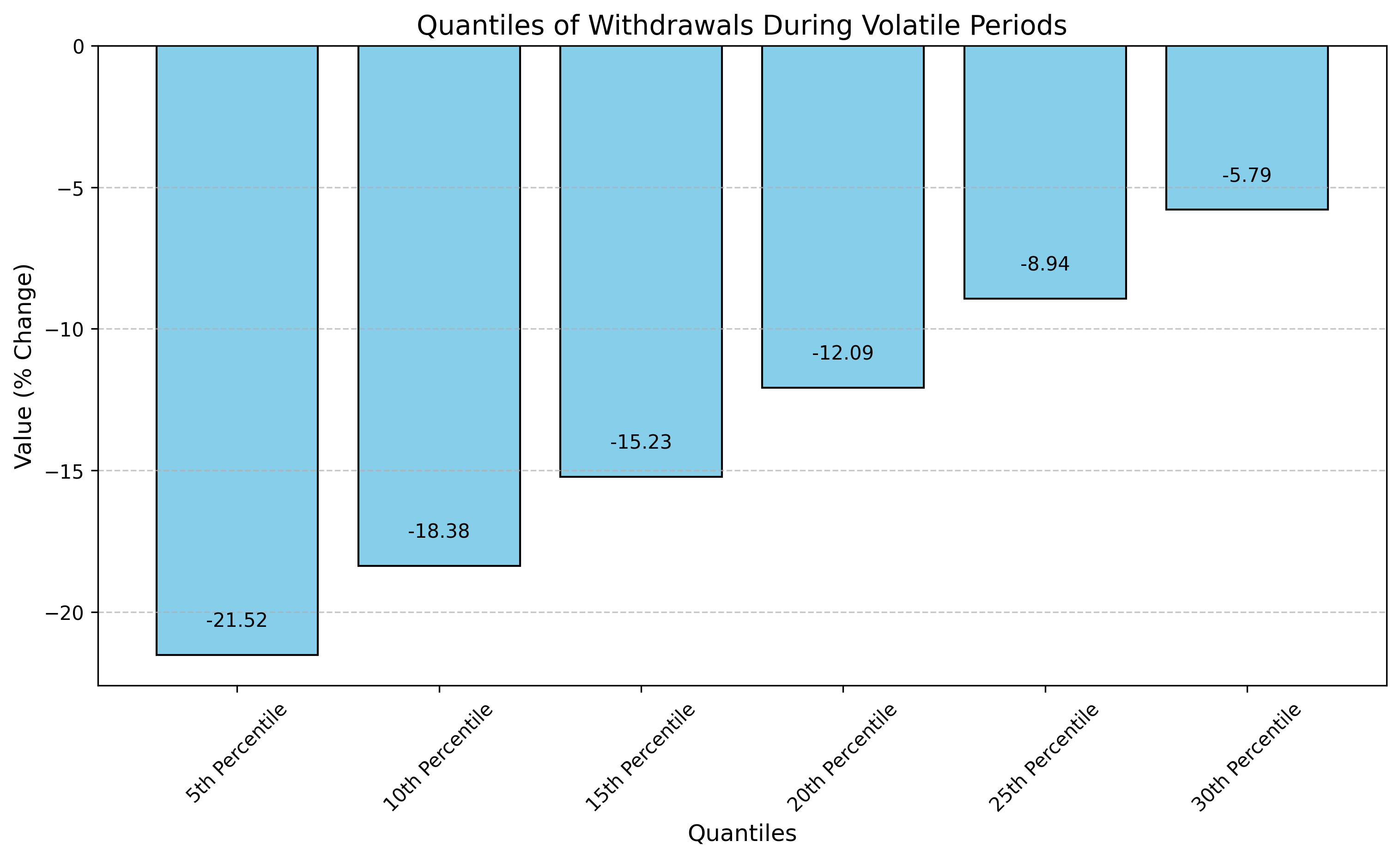
The 10th percentile of negative withdrawals of supplied crvUSD during volatile periods was 18% of the total supply.This means that 90% of all observed withdrawals during volatile periods were less than or equal to this value. Given that optimal utilization is defined as min(1- withdrawal_quantile, 0.85), optimal utilization is 82%.
 Regime Shift Analysis
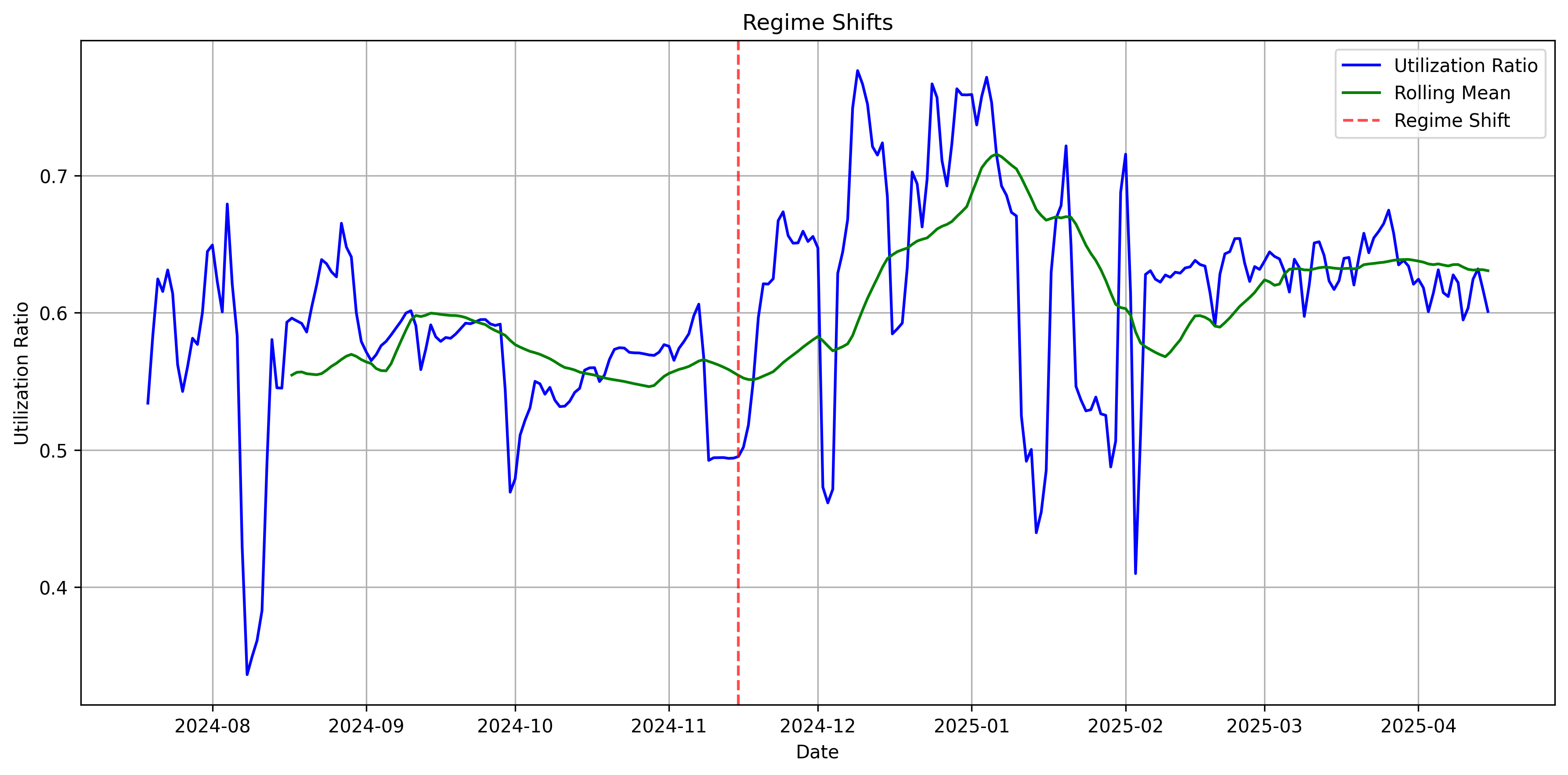
This plot shows detected regime shifts in utilization. Red vertical lines indicate significant shifts, which represents changes in stability in utilization in this given market. While the CRV market did not undergo a regime shift since our last analysis, re-running the analysis is needed and should yield different results as the level of optimal utilization changes.
In order to validate with the latest parameter, we select the sub-section of this regime where the latest updated parameter were implemented. Hence, we utilize the data from the 2025-02-19 to 2025-04-14, covering a period of 54 days.
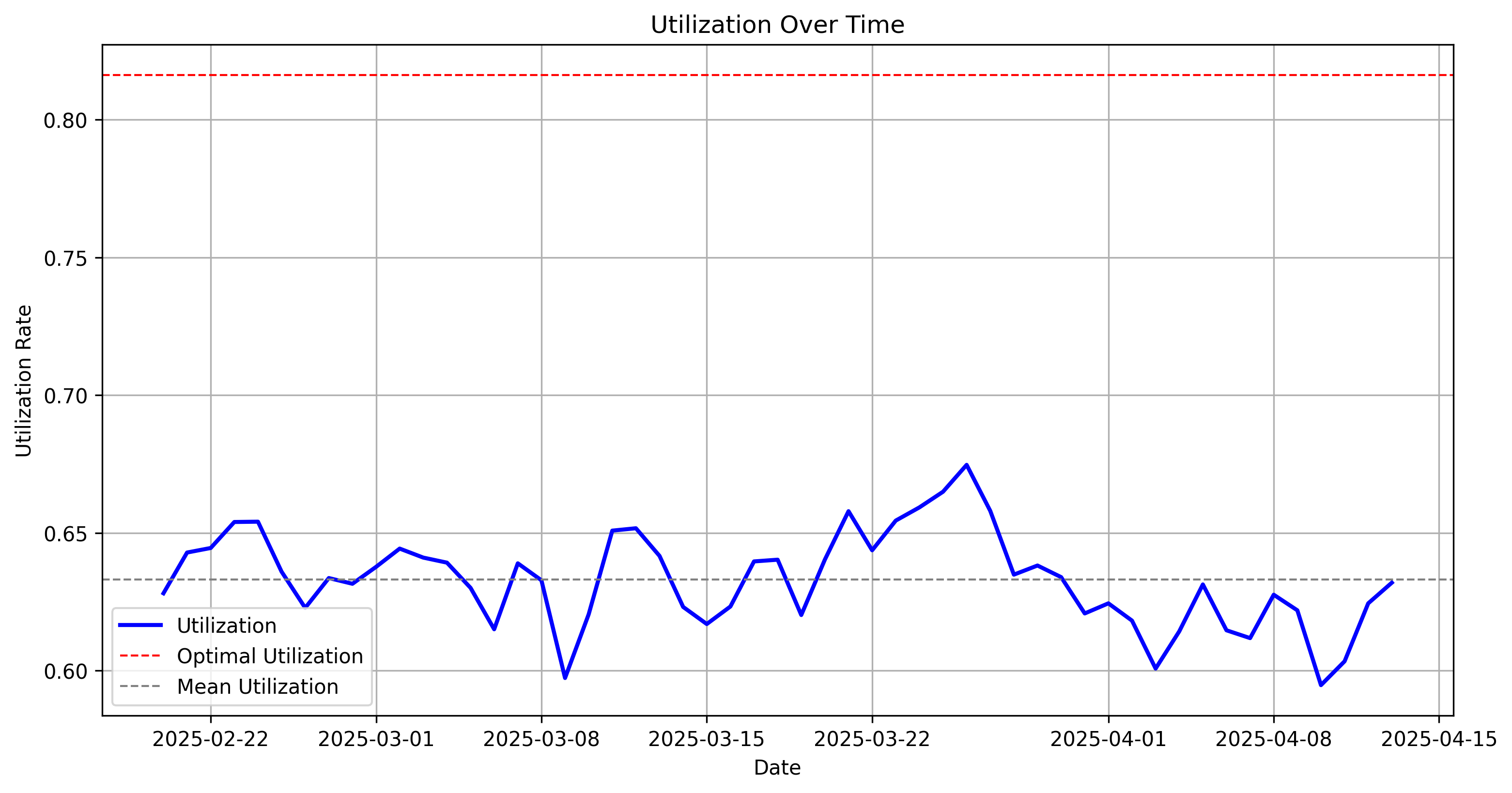
The regime, given the new level of optimal utilization, can now be considered underutilized.
Validation of the underlying Model for the SDE
OLS Regression Results
==============================================================================
Dep. Variable:      delta_utilization   R-squared:                       0.158
Model:                            OLS   Adj. R-squared:                  0.141
Method:                 Least Squares   F-statistic:                     9.183
Date:                Tue, 15 Apr 2025   Prob (F-statistic):            0.00389
Time:                        18:04:23   Log-Likelihood:                 151.08
No. Observations:                  51   AIC:                            -298.2
Df Residuals:                      49   BIC:                            -294.3
Df Model:                           1
Covariance Type:            nonrobust
==================================================================================
                     coef    std err          t      P>|t|      [0.025      0.975]
----------------------------------------------------------------------------------
const              0.0333      0.011      3.060      0.004       0.011       0.055
borrow_apr_lag    -0.2358      0.078     -3.030      0.004      -0.392      -0.079
==============================================================================
Omnibus:                        0.744   Durbin-Watson:                   1.649
Prob(Omnibus):                  0.689   Jarque-Bera (JB):                0.849
Skew:                          -0.216   Prob(JB):                        0.654
Kurtosis:                       2.539   Cond. No.                         44.4
==============================================================================

Notes:
[1] Standard Errors assume that the covariance matrix of the errors is correctly specified.
Validating the Underlying Model
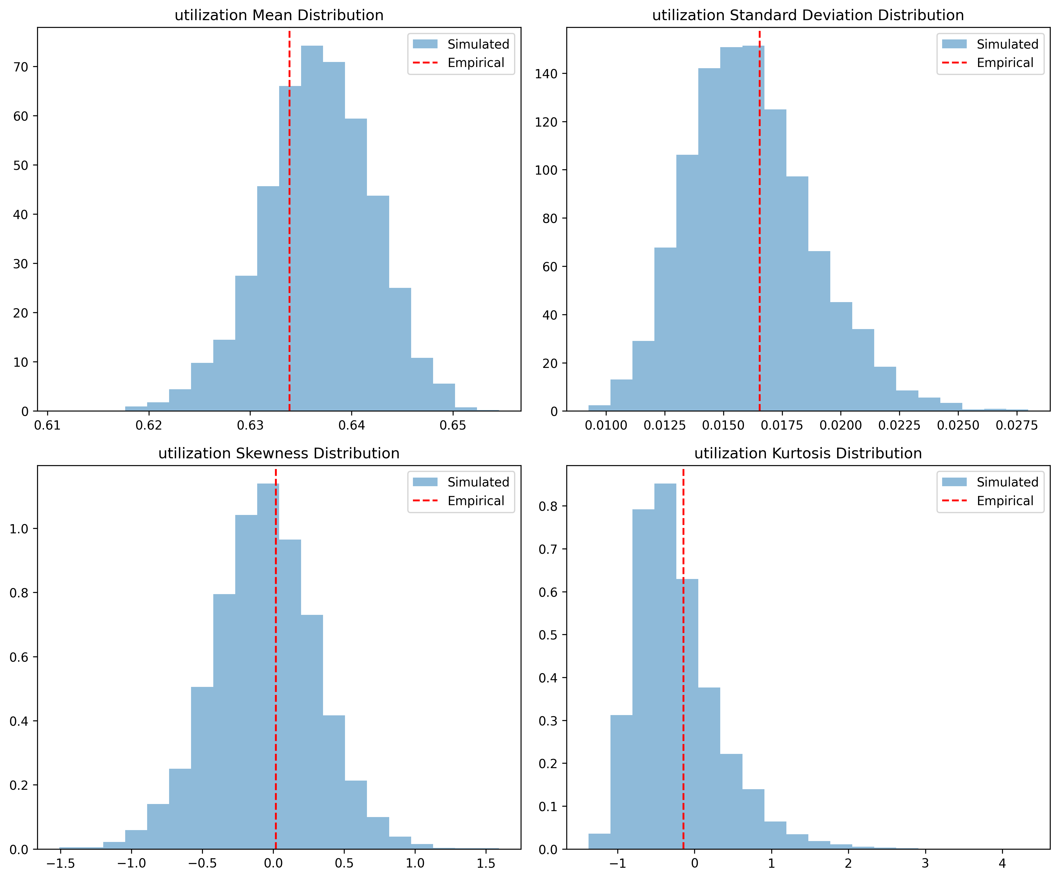
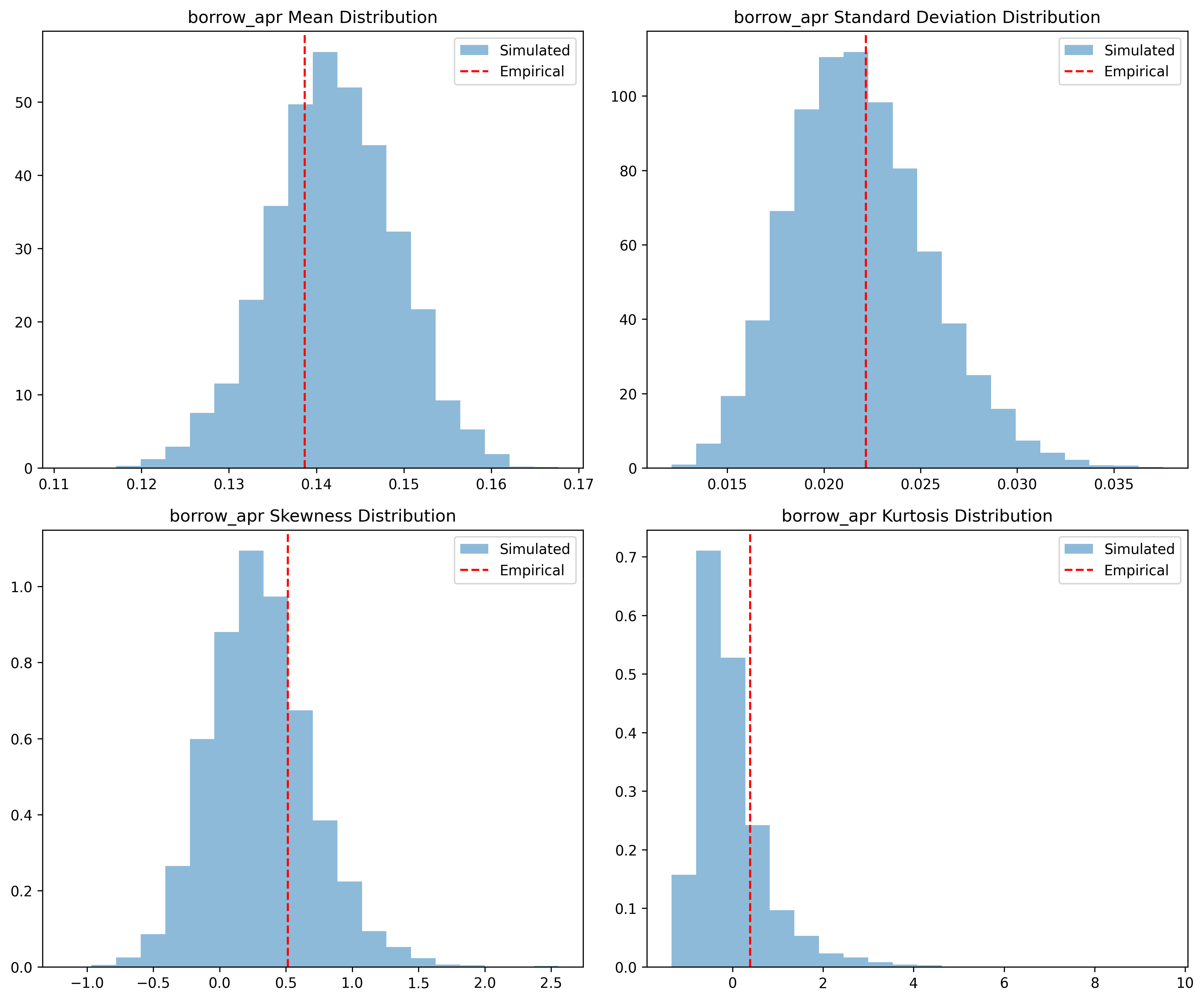
This plot visualizes the distribution of key statistical metrics for empirical vs. simulated utilization. Red lines mark empirical mean values, allowing direct comparison with simulated distributions.
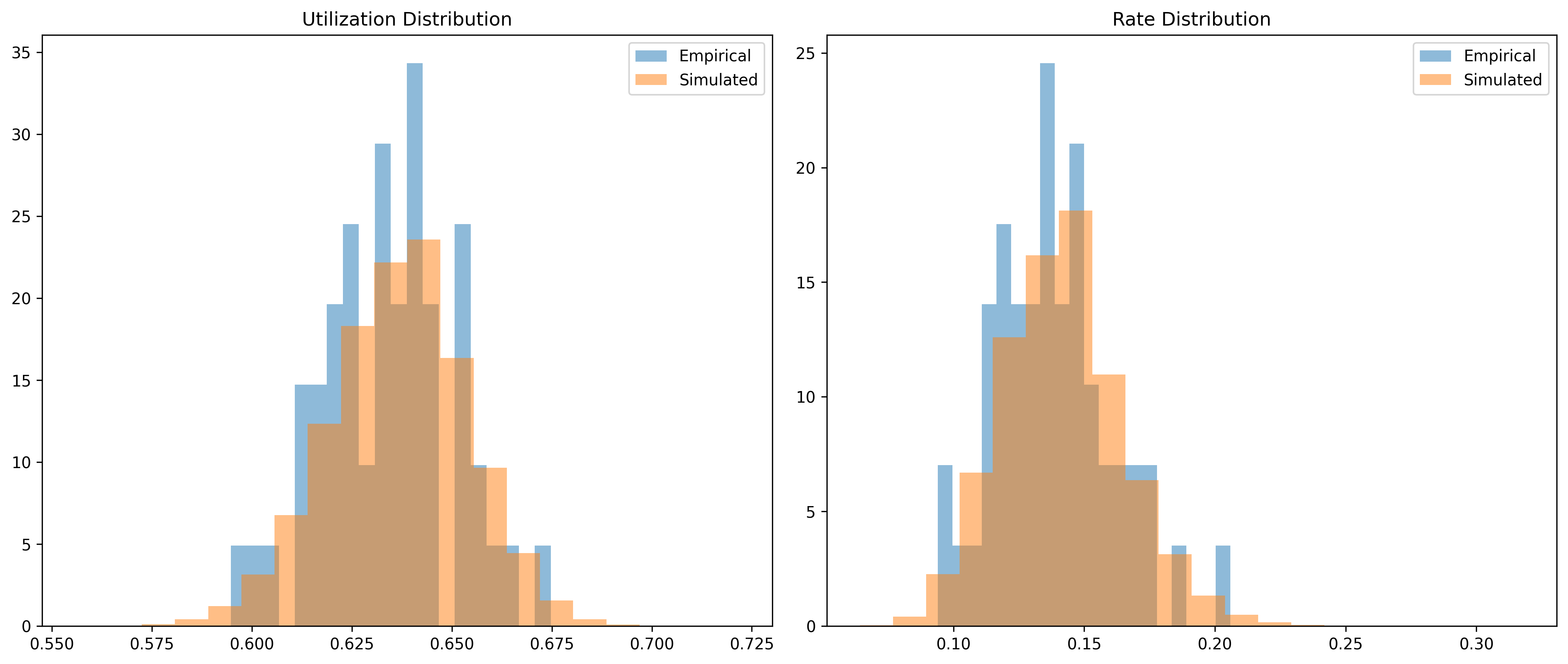
This plot compares the empirical and simulated distributions of utilization and rates. A close match indicates realistic simulation dynamics.
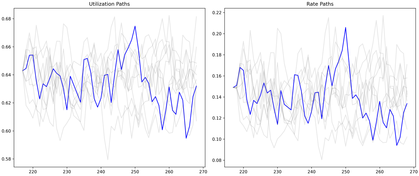
This plot compares real utilization and rate paths with simulated ones. Gray lines represent simulated paths, while blue lines show empirical values.
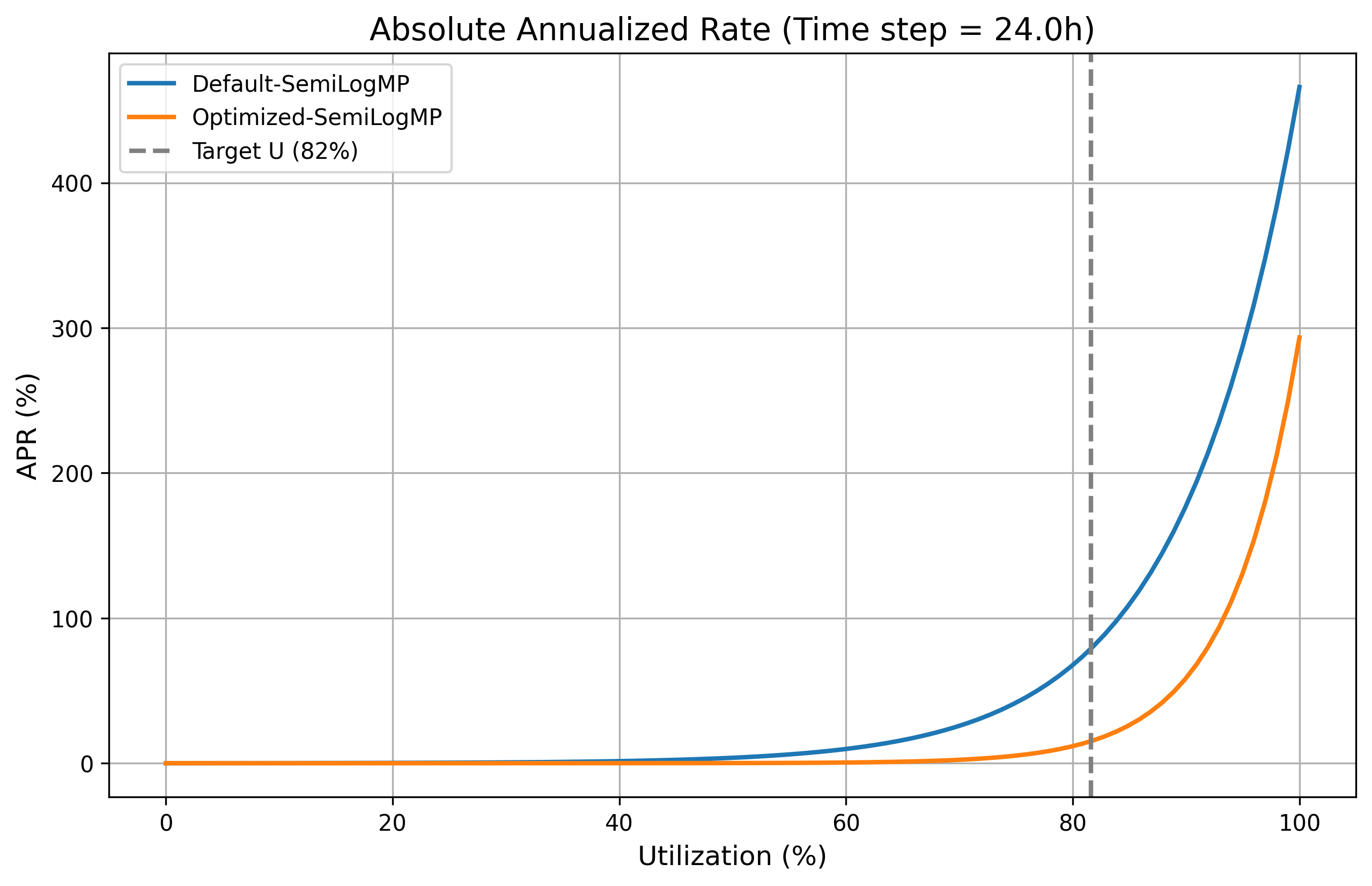
Identifying Optimal Parameters
After optimizing with the composite loss function across multiple simulated SDE paths, we identified the optimal parameters as:
| IRM Label | Parameter | Optimized Value |
|---|---|---|
Optimized-SemiLogMP |
rate_min |
3e-07 |
Optimized-SemiLogMP |
rate_max |
2.93384 |
Evaluation of Optimized Model
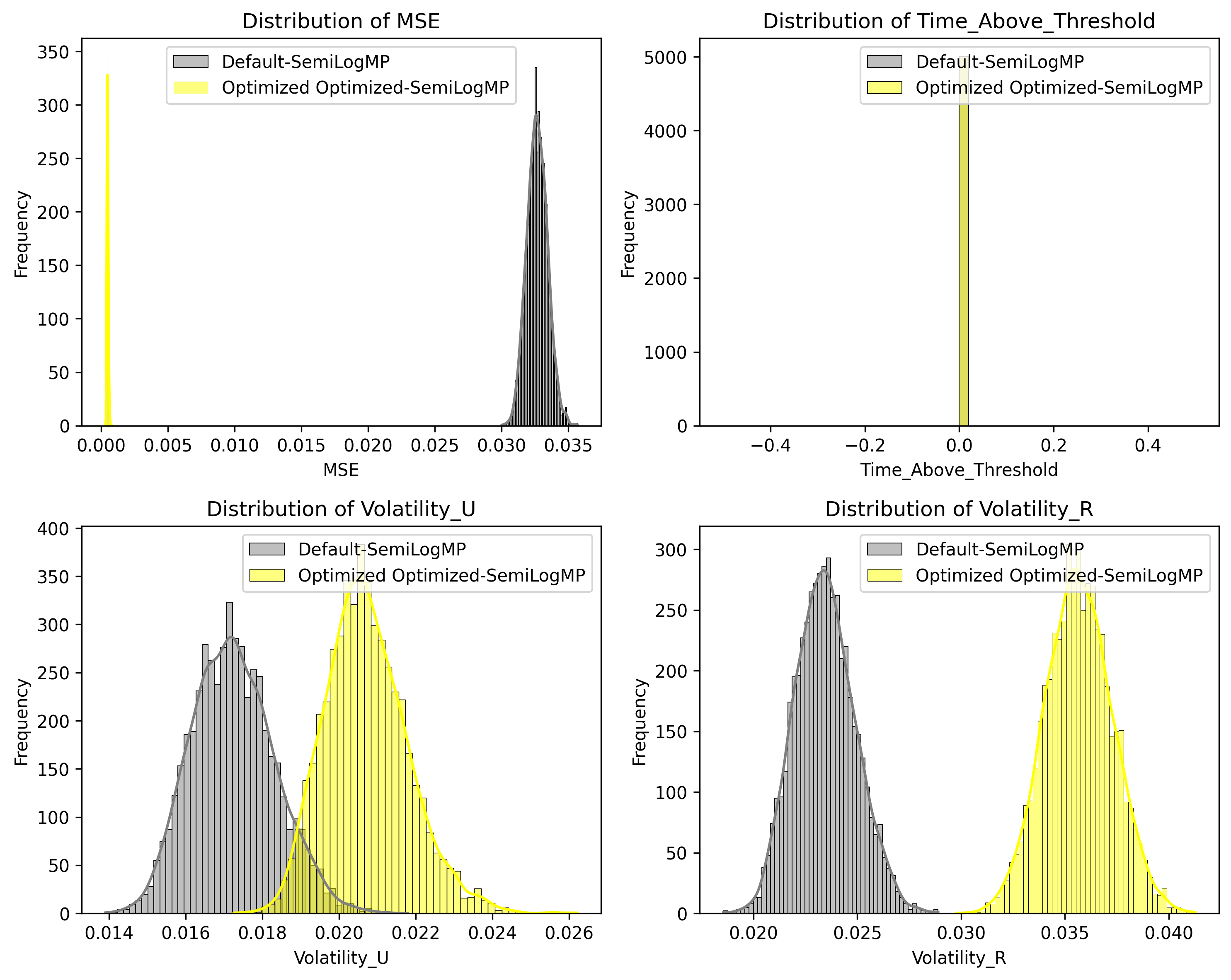
Unsurprisingly, we expect the new model parameters to perform meaningfully better. This is indicated by a substantially lower Mean-squared Error (MSE) in the optimized configuration compared to the existing configuration.
Specification:
ACTIONS = [
    # Set CRV-long Params
    ("0x8a7138cF49AffCd35D05dBE5a160Dac870E4B6F5", "set_rates", 5761669, 137947108067),
]